Posts

Jul 17, 2025

Conv2D GPU Baselines: cuDNN and CUTLASS Performance and Analysis (Part 2)

Categories:CUDA,CPU

In Part 1: Tuning Conv2D from CPU to GPU from Scratch, we optimized a convolutional kernel from a naive nested loop on CPU to a multi-threaded NHWC version with OpenMP, bringing runtime from 150 seconds to 3.4 seconds.

Now, we turn to the GPU and ask: how fast can industry-standard libraries like cuDNN and CUTLASS make this kernel? And how much of the GPU’s peak compute can they actually use?

Below, we’ll benchmark both libraries, analyze their internals with Nsight Compute, and compare them against the theoretical peak we calculated in Part 1.

Table of Contents

1. Why Use cuDNN and CUTLASS
2. Benchmark Setup
3. Results: cuDNN vs CUTLASS
4. What’s Under the Hood?
5. Performance Summary So Far
6. What’s Next?
7. Appendix

Why Use cuDNN and CUTLASS

cuDNN

cuDNN is NVIDIA’s production-grade GPU library used by most deep learning frameworks (PyTorch, TensorFlow). It’s hand-tuned for every GPU generation and uses advanced algorithms like:

• Winograd convolution
• Implicit GEMM
• Tensor Core acceleration
• Kernel auto-tuning for each shape

As cuDNN is closed source, we can only infer their operation via metrics that NSight profile reveals.

CUTLASS

CUTLASS is an open-source CUDA C++ template library developed by NVIDIA. At its core is a collection of abstractions for implementing high-performance GEMM and convolution kernels on GPUs.

One of its core components is CuTe (CUDA Tensor), which provides tensor views with fine-grained control over layout, shape, and tiling. Instead of manually computing strides or worrying about memory bank conflicts, you can declaratively specify how tensor elements should map across threads, warps, and threadblocks in a memory-efficient way.

The general idea of CUTLASS in implementing a Convolution kernel is it provides high parameterized C++ CUDA templates. It decomposes the kernel into the following parts,

• Input & weight iterators: for coalesced shared memory loads
• Implicit GEMM mapping: to transform NHWC × KRSC into GEMM tiles
• Device-specific MMA ops: using CUDA or Tensor Cores
• Epilogue: to store accumulator registers into global memory efficiently

We’ll use CUTLASS and cuDNN for benchmarking against how well they perform on my platform. And CUTLASS as the framework we’ll gradually deconstruct in future posts.

Benchmark Setup

We used the same Conv2D configuration:

Parameter	Value
Input	NHWC (10, 224, 224, 128)
Filter	KRSC (128, 3, 3, 128)
Output	(10, 224, 224, 128)
Padding	1
Stride	1
Dilation	1
Data type	FP32, FP16
Device	NVIDIA RTX 2070 Super

We benchmarked:

• cuDNN in both NCHW and NHWC formats.
• CUTLASS with SIMT (FPU) and Tensor Core (FP16) kernels.

Results: cuDNN vs CUTLASS

Library	Layout	Algo	Data Type	Time (ms)	% of Theoretical Peak*
cuDNN	NCHW	Winograd	FP32	15.94 ms	100.4 %
cuDNN	NHWC	Winograd	FP32	17.15 ms	93.3 %
CUTLASS	NHWC	CUDA Core	FP32	27.96 ms	43.4 %
CUTLASS	NHWC	Tensor Core	FP16	6.23 ms	32.1 %

* Theoretical peak: 16 ms (FP32 CUDA core), 2 ms (FP16 Tensor Core), from Part 1

It may seem surprising that cuDNN appears to exceed the theoretical peak of 16 ms. But this is due to the fact that cuDNN’s Winograd implementation does not compute a full 3×3 convolution directly. Which transforms the problem into a compressed domain where the number of multiplications is greatly reduced.

Let’s take a digression to measure how many fp32 instruction cuDNN saved from using Winograd.

Digression: Winograd vs Direct Convolution Flops count

We can do so by using NSight to get the number of FMA ops it performs. Recall that in Part 1, we calculated the number of FMA ops as N*P*Q*K*C*R*S = 73.987 billion. Let’s verify that a naive convolution performs that many ops, using

ncu --metrics smsp__sass_thread_inst_executed_op_fp32_pred_on.sum

  manual_conv2d_kernel(const float *, const float *, float *, int, int, int, int, int, int, int, int, int, int, int, int, int, int, int, int, int) (3920, 1, 2)x(256, 1, 1), Context 1, Stream 7, Device 0, CC 7.5
    Section: Command line profiler metrics
    --------------------------------------------------- ----------- --------------
    Metric Name                                         Metric Unit   Metric Value
    --------------------------------------------------- ----------- --------------
    smsp__sass_thread_inst_executed_op_fp32_pred_on.sum        inst 74,836,500,480
    --------------------------------------------------- ----------- --------------

We see that the total FP32 op executed on a naive Conv2D kernel is very close to our calculated FMA op counts, at 74.0 and 74.8 billion ops respectively.

Next, we measure the number of FP32 ops performed by cuDNN,

Kernel	Op Count (Billions)
Winograd Forward Data 4x4	1.233
Winograd Forward Filter 4x4	0.001
Volta SGEMM 128x64 NN	29.830
Winograd Forward Output 4x4	1.355
Total cuDNN	32.419

Based on this reduced operation count (~32.4 billion ops total after including transforms), cuDNN’s effective compute workload is about 43% of direct Conv2D. This means its actual peak runtime should be 6.91 ms — not 16 ms — making its real utilization ~43.4%.

Library	Layout	Algo	Data Type	Time (ms)	% of Theoretical Peak*
cuDNN	NCHW	Winograd	FP32	15.94 ms	43.4 %
cuDNN	NHWC	Winograd	FP32	17.15 ms	40.3 %
CUTLASS	NHWC	CUDA Core	FP32	27.96 ms	43.4 %
CUTLASS	NHWC	Tensor Core	FP16	6.23 ms	32.1 %

What’s Under the Hood?

Library	Algorithm	Layout	Tensor Cores	Tiling
cuDNN	Winograd	NHWC	Yes	Dynamic (opaque)
CUTLASS	Implicit GEMM	NHWC	Optional	Explicit templates

For example, in CUTLASS:

• Tensor Core kernels use fragments (mma.sync) over shared memory tiles.
• CUDA Core (SIMT) kernels use FMA loops over global/shared memory tiles.
• All kernels follow a load → compute → epilogue pipeline.

Performance Summary So Far

Version	Time	Speedup over CPU	% of Peak attainable
Naive CPU	150 s	1×	0.24
CPU (NHWC + OMP)	3.4 s	44×	10.6
cuDNN NCHW	15.9 ms	9,434x	43.4
cuDNN NHWC	17.2 ms	8,721x	40.3
CUTLASS SIMT	28 ms	5,357x	43.4
CUTLASS Tensor	6.2 ms	24,194×	32.1

What’s Next?

cuDNN and CUTLASS are fast - but how do they actually work?

In the next posts, we’ll build a Conv2D CUDA kernel from scratch, mimicking CUTLASS pipeline:

• shared memory staging
• threadblock tiling
• register-level accumulation
• split-k gemm tiling
• epilogue accumulation and write back

Our goal is to build a bare-metal CUDA kernel — without any external header — that matches or even exceeds the hardware efficiency of these production-grade libraries.

By writing our own Conv2D kernel from scratch, we’ll better understand:

• Where real GPU performance comes from,
• How tiling and memory staging impact latency,
• And what it really takes to hit 40%+ of peak performance.

Appendix:

We include the grid and block size for the various kernels before, and briefly highlight their notable features,

cuDNN NCHW (15.94 ms)

Function Name	Grid Size	Block Size	Duration [msecond]
vectorized_elementwise_kernel	62720, 1, 1	128, 1, 1	0.93
vectorized_elementwise_kernel	144, 1, 1	128, 1, 1	0.01
winogradForwardData4x4	196, 128, 1	256, 1, 1	3.94
winogradForwardFilter4x4	4, 16, 1	32, 8, 1	0.01
volta_sgemm_128x64_nn	392, 2, 36	128, 1, 1	8.19
winogradForwardOutput4x4	196, 128, 1	256, 1, 1	2.86

cuDNN performs a Winograd transform on the input and filter, applies GEMM, and then transforms the output back from the Winograd domain.

cuDNN NHWC (17.15 ms)

Function Name	Grid Size	Block Size	Duration [msecond]
vectorized_elementwise_kernel	62720, 1, 1	128, 1, 1	0.93
vectorized_elementwise_kernel	144, 1, 1	128, 1, 1	0.01
nhwcToNchwKernel	1568, 4, 10	256, 1, 1	1.41
nhwcToNchwKernel	1, 4, 128	256, 1, 1	0.01
generateWinogradTilesKernel	4, 32, 1	32, 4, 1	0.01
_5x_cudnn_volta_scudnn_winograd_128x128_ldg1_ldg4_relu_tile148t_nt_v1	40, 28, 14	256, 1, 1	13.30
nchwToNhwcKernel	1568, 4, 10	256, 1, 1	1.48

Here, cuDNN is actually transforming NHWC into NCHW before performing winograd.

This is somewhat surprising, as NHWC is typically considered more optimal for GPU memory access. However, it suggests that cuDNN’s Winograd kernels may be optimized specifically for NCHW, and the overhead of layout transformation is worth the tradeoff.

CUTLASS CUDA Core (27.96 ms)

Function Name	Grid Size	Block Size	Duration [msecond]
vectorized_elementwise_kernel	62720, 1, 1	128, 1, 1	0.93
vectorized_elementwise_kernel	144, 1, 1	128, 1, 1	0.00
vectorized_elementwise_kernel	62720, 1, 1	128, 1, 1	0.63
Kernel	3920, 1, 1	256, 1, 1	26.40

CUTLASS provides a clean implicit GEMM kernel via DefaultConv2dFprop. With float32 data and SIMT path, we reach 28 ms. Although this is slower than cuDNN, accounting for the reduced operation count in cuDNN’s Winograd implementation reveals that both achieve similar hardware utilization — around 43.4% of theoretical peak.

CUTLASS Tensor Core (6.23 ms)

Function Name	Grid Size	Block Size	Duration [msecond]
vectorized_elementwise_kernel	62720, 1, 1	128, 1, 1	0.95
vectorized_elementwise_kernel	144, 1, 1	128, 1, 1	0.00
vectorized_elementwise_kernel	62720, 1, 1	128, 1, 1	0.32
Kernel	1960, 1, 1	256, 1, 1	4.96

By switching to __half types and enabling Tensor Core kernels, CUTLASS hits 6.23 ms — the fastest kernel among all tested configurations. However, its hardware utilization is the lowest at 28.9%.

Jul 12, 2025

Optimizing Conv2D from Scratch: CPU to GPU Journey (Part 1)

Categories:CUDA,CPU

In this blog series, I’ll walk through my journey optimizing a canonical Conv2D kernel — starting from a deeply nested CPU loop, all the way to handcrafted CUDA kernels that rival cuDNN and CUTLASS.

Table of Contents

1. Motivation
2. Background: What Does Conv2D Actually Do?
3. Roofline: Theoretical Peak Performacne
4. CPU Implementation and Tuning
5. What’s Next

Motivation

The convolution layer is the cornerstone of modern neural networks. This series documents the engineering path from naive to state-of-the-art implementations of a Conv2D operation — measuring the work, insight, and tooling required to bridge the performance gap.

We chose a canonical configuration:

• Input: NHWC shape (10, 224, 224, 128)
• Filter: KRSC shape (128, 3, 3, 128)
• Output: NPQK shape (10, 224, 224, 128)
• Padding: 1, Stride: 1, Dilation: 1

This setup represents a mid-depth convolutional layer common in real-world CNNs (e.g., EfficientNet, ResNet), and its optimization is relevant for both training and inference pipelines.

Background: What Does Conv2D Actually Do?

At its core, a 2D convolution computes weighted dot products over local spatial windows across input channels. Here’s a visualization with a 3×3 kernel. Imagine each 3×3 input patch has a depth of C = 128. Each filter produces a single output value, and we use K = 128 such filters. This gives a filter shape of KRSC = (128, 3, 3, 128).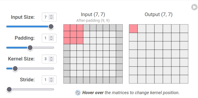



Credit: https://poloclub.github.io/cnn-explainer/

Mathematically, for each output element O[n, p, q, k], we compute:

\[O[n, p, q, k] = \sum_{r = -1}^{1} \sum_{s = -1}^{1} \sum_{c = 0}^{C - 1} I[n, p + r, q + s, c] \cdot W[k, r + 1, s + 1, c]\]

Note: r and s range from -1 to 1 due to centered 3×3 kernels.

Roofline: Theoretical Peak Performance

Before diving into code, we estimate the ideal performance bounds on our hardware to benchmark how close our implementation gets to peak throughput.

We start by analyzing arithmetic intensity (AI) — the ratio of computation to memory traffic. This tells us whether the kernel is compute-bound or memory-bound.

Arithmetic Intensity (AI) Analysis of Conv2D

Total Floating Point Operations (FLOPs)

Each output element performs:

• CRS = 128 × 3 × 3 = 1152 multiply-accumulates
• Each MAC = 2 FLOPs

Total FLOPs:

\[\text{FLOPs} = N \times P \times Q \times K \times C \times R \times S \times 2 = 147.975 \text{ GFLOPs}\]

---

Total Memory Accessed

Unique elements accessed:

• Input (NHWC): 10 × 224 × 224 × 128 = 64,100,352
• Filter (KRSC): 128 × 3 × 3 × 128 = 147,456
• Output (NPQK): 10 × 224 × 224 × 128 = 64,100,352

Total: 128,598,160 elements

• FP32: 128,598,160 × 4 bytes = 514.39 MB
• FP16: 128,598,160 × 2 bytes = 257.20 MB

---

Arithmetic Intensity (AI)

• FP32: 147.975 GFLOPs / 514.39 MB = 287.67 FLOP/byte
• FP16: 147.975 GFLOPs / 257.20 MB = 575.34 FLOP/byte

---

Roofline: CPU vs GPU

CPU: AMD Ryzen 2700

Spec	Value
Cores	8 (SMT disabled)
Clock speed	3.2 GHz
SIMD width	AVX2 (8 FP32 per register)
Peak FLOPs	409.6 GFLOP/s
Mem bandwidth (DDR4-3200)	~51.2 GB/s
Ridge Point	8.0 FLOP/byte

GPU: RTX 2070 Super (CUDA Cores)

Spec	Value
SMs	40
CUDA cores per SM	64
Clock speed	1.8 GHz
Peak FLOPs	9.216 TFLOP/s
Mem bandwidth	448 GB/s
Ridge Point	20.57 FLOP/byte

GPU: RTX 2070 Super (Tensor Cores)

Spec	Value
Tensor cores (40 SMs × 8)	320
Peak FLOPs (FP16)	73.728 TFLOP/s
Ridge Point	164.57 FLOP/byte

---

Conclusion

In all cases, the kernel AI is well above each device’s ridge point, which means:

• The kernel is compute-bound on both CPU and GPU.
• We can estimate ideal runtimes by dividing FLOPs by peak device throughput:

Device	Peak FLOP/s	Ideal Time
Ryzen 2700	409.6 GFLOP/s	361 ms
RTX 2070 (CUDA)	9.216 TFLOP/s	16.05 ms
RTX 2070 (Tensor)	73.728 TFLOP/s	2.01 ms

---

CPU Implementation and Tuning

Naive CPU Kernel (NCHW Layout)

Our initial implementation used NCHW and ran in 150 seconds — far from the ideal 361 ms.

extern "C" void conv2d(float* input, float* weight, 
                       int n,
                       int h, int w, int c_in,
                       int r, int c_out,
                       int stride,
                       int padding,
                       float* z)
{
    int p = (h + 2*padding - r) / stride + 1;
    int q = (w + 2*padding - r) / stride + 1;

    const int r_offset = (r - 1) / 2;
    const int s_offset = (r - 1) / 2;

    for (int n_i = 0; n_i < n; ++n_i) {
        for (int k_i = 0; k_i < c_out; ++k_i) {
            for (int p_i = 0; p_i < p; ++p_i) {
                for (int q_i = 0; q_i < q; ++q_i) {
                    float acc = 0;

                    for (int c_i = 0; c_i < c_in; ++c_i) {
                        for (int r_i = 0; r_i < r; ++r_i) {

                            int h_i = p_i + r_i - r_offset;
                            if (h_i < 0 || h_i >= h) continue;

                            for (int s_i = 0; s_i < r; ++s_i) {

                                int w_i = q_i + s_i - s_offset;
                                if (w_i < 0 || w_i >= w) continue;

                                int input_index = ((n_i * c_in + c_i) * h + h_i) * w + w_i;
                                int weight_index = ((k_i * c_in + c_i) * r + r_i) * r + s_i;

                                acc += input[input_index] * weight[weight_index];
                            }
                        }
                    }

                    int output_index = ((n_i * c_out + k_i) * p + p_i) * q + q_i;
                    z[output_index] = acc;
                }
            }
        }
    }
}

Improving Cache Locality with NHWC

Switching to NHWC and restructuring loops around the innermost C dimension brought runtime down to 23 seconds — a 6.5× speedup due to better memory locality.

extern "C" void conv2d_nhwc(float* __restrict__ input, float* __restrict__ weight, 
                            int n,
                            int h, int w, int c_in,
                            int r, int c_out,
                            int stride,
                            int padding,
                            float* __restrict__ z)
{
    int p = (h + 2*padding - r) / stride + 1;
    int q = (w + 2*padding - r) / stride + 1;

    const int r_offset = (r - 1) / 2;
    const int s_offset = (r - 1) / 2;

    for (int n_i = 0; n_i < n; ++n_i) {
        for (int p_i = 0; p_i < p; ++p_i) {
            for (int q_i = 0; q_i < q; ++q_i) {
                for (int k_i = 0; k_i < c_out; ++k_i) {

                    float acc = 0;

                    for (int r_i = 0; r_i < r; ++r_i) {

                        int h_i = p_i + r_i - r_offset;
                        if (h_i < 0 || h_i >= h) continue;

                        for (int s_i = 0; s_i < r; ++s_i) {

                            int w_i = q_i + s_i - s_offset;
                            if (w_i < 0 || w_i >= w) continue;

                            for (int c_i = 0; c_i < c_in; c_i += 8) {

                                int input_index = ((n_i * h + h_i) * w + w_i) * c_in + c_i;
                                int weight_index = ((k_i * r + r_i) * r + s_i) * c_in + c_i;

                                float tmp_acc = 0;

                                for (int c_offset = 0; c_offset < 8; ++c_offset) {
                                    tmp_acc += input[input_index + c_offset] * weight[weight_index + c_offset];
                                }
                                acc += tmp_acc;
                            }
                        }
                    }

                    int output_index = ((n_i * c_out + k_i) * p + p_i) * q + q_i;
                    z[output_index] = acc;
                }
            }
        }
    }
}

Adding OpenMP Parallelism

By parallelizing over the outer loops (e.g., n, p, q), we utilized 8 physical CPU cores:

    #pragma omp parallel for collapse(2) schedule(static)
    for (int n_i = 0; n_i < n; ++n_i) {
        for (int p_i = 0; p_i < p; ++p_i) {
            for (int q_i = 0; q_i < q; ++q_i) {
                for (int k_i = 0; k_i < c_out; ++k_i) {
                    ...

This further reduced runtime to 3.4 seconds, a 44× overall improvement.

Summary: CPU Conv2D Performance

Version	Layout	Parallelism	Time	Speedup
Naive CPU	NCHW	None	150 s	1×
Naive CPU	NHWC	None	23 s	6.5×
CPU + OMP	NHWC	8 cores	3.4 s	44×

This final CPU implementation achieved about 11% of theoretical peak, which is quite reasonable for a memory-coordinated workload without heavy vectorization or compiler intrinsics.

What’s next?

In Part 2, we’ll explore cuDNN and CUTLASS baselines on the GPU, and eventually challenge them with our own hand-rolled CUDA kernels.

The big question: How hard is it to get from 3.4 seconds down to 2.01 ms

Feb 26, 2025

Deepseek V3/R1 intra/inter node all-to-all communication

Categories:CUDA

Recently, DeepSeek V3 made headlines by being able to train 14.8 trilion tokens using only 2.788 million H800 GPU hours. This was estimated to be several times more efficient than approaches that did not incorporate DeepSeek’s LLM and training infrastructure designs.

In the initial 2024-12-26 announcement for DeepSeek-V3, and subsequently the publishing of the inference repo, one part that remained missing stood out to me; which is on how the cross GPU communication kernels are implemeneted.

3.2.2. Efficient Implementation of Cross-Node All-to-All Communication

… In detail, we employ the warp specialization technique (Bauer et al., 2014) and partition 20 SMs into 10 communication channels. During the dispatching process, (1) IB sending, (2) IB-to-NVLink forwarding, and (3) NVLink receiving are handled by respective warps. The number of warps allocated to each communication task is dynamically adjusted according to the actual workload across all SMs. Similarly, during the combining process, (1) NVLink sending, (2) NVLink-to-IB forwarding and accumulation, and (3) IB receiving and accumulation are also handled by dynamically adjusted warps. In addition, both dispatching and combining kernels overlap with the computation stream, so we also consider their impact on other SM computation kernels. Specifically, we employ customized PTX (Parallel Thread Execution) instructions and auto-tune the communication chunk size, which significantly reduces the use of the L2 cache and the interference to other SMs.

From the quote above in their paper, I’m also curious about what customized PTX instructions are used. Given that these are missing in their repo, I suspected it was a secret sauce that they didn’t intend to share.

Fortunately, I was proven wrong as the DeepSeek team published the DeepEP repo on 2025-02-26.

Thus my post below will attempt to analyze the key designs in the communication kernel.

Table of Contents

1. The Problem: Scalable MoE in LLMs
2. Key Design Choices for Efficient Communication
3. Communication Kernel Implementation Details
4. Appendix

The Problem: Scalable MoE in LLMs

Modern large language models (LLMs) started introducing a layer called “Mixture of Experts” (MoE) in their Transformer blocks to scale parameter count without linearly increasing compute. This is typically done through top-k (often k=2) “expert routing”, where each token is dispatched to two specialized feed-forward networks (experts) out of a large pool.

A naive GPU cluster implementation would be to place each expert on a separate device and have the router dispatch to the selected experts during inference. But this would have all the non-active experts idle on the expensive GPUs.

GShard, 2021 introduced the concept of sharding these feed-forward (FF) experts across multiple devices, so that each device:

1. Processes a partition of tokens (a token “group”), computing gating scores (often with softmax) to decide which experts these tokens should go to.
2. Dispatches embeddings to remote devices that host the relevant experts.
3. Combines the outputs from those experts, which are sent back from other devices, before proceeding to the next layer in the Transformer.

This diagram from GShard paper illustrates how the cross device communication happen



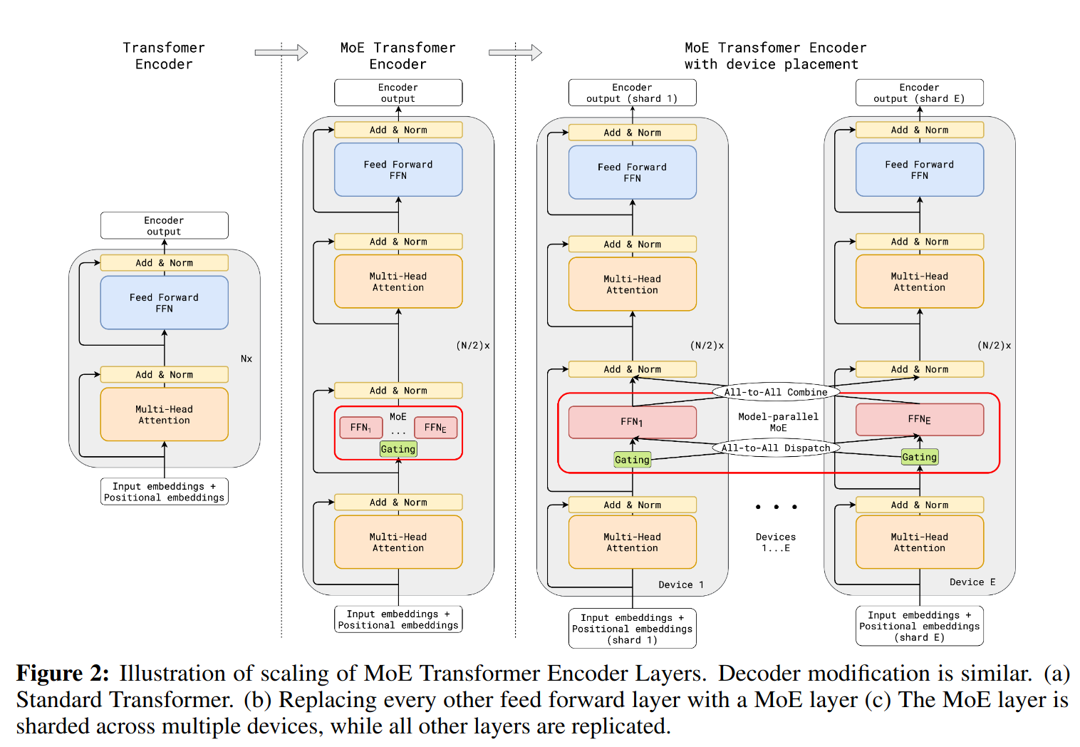
• It is worth clarifying that the transformer block in each shard is processing the full token embedding, thus the attention itself are complete and do not depend on other shards. It is only the [tokens, channels] going into each shard’s FF need to be assembled from tokens coming from remote devices. I think of each shard’s group tokens as a mini-batch in itself.

The challenge: all-to-all communication

Each device must send chunks of embeddings to potentially every other device (intra-node via NVLink, inter-node via InfiniBand RDMA). If done naively, this quickly becomes a communication bottleneck. DeepSeek’s DeepEP addresses this with specialized CUDA kernels that optimize dispatch and combine steps for both inter- and intra-node traffic, while also seamlessly overlapping communication with local compute to hide each other’s latency.

Key Design Choices for Efficient Communication

DeepEP’s performance gains revolve around carefully orchestrating the overlap of communication and compute while optimizing low-level CUDA operations for the specific MoE data patterns.

1. Dual-Stream execution

   Each device runs two CUDA streams in parallel:

   • Compute Stream: Handles attention, softmax, feed-forward, and layer normalization for the local tokens
   • Communication Stream: Handles all the dispatch/combine operations for MoE.

   By running both streams concurrently, together with careful scheduling, DeepSeek claims to

   This overlap also ensures that, as the model further scales up, as long as we maintain a constant computation-to-communication ratio, we can still employ fine-grained experts across nodes while achieving a near-zero all-to-all communication overhead

2. Hand-Rolled CUDA Extensions

   DeepEP provides a custom deep_ep.cpp CUDA extension with an API that combines:

   • Intra-node NVLink communication kernel for MoE dispatch/combine
   • Inter-node InfiniBand RDMA

   This allows fine-grained control over reading/writing GPU memory for dispatch and combine. By tailoring these kernels to MoE’s all-to-all pattern, they avoid generic overhead and can exploit hardware features like warp-specialized loops, ring buffers, and pinned memory.

3. Using out-of-doc PTX instruction to minimize interference between the Communication and Computation stream

   To reduce L1 cache thrashing, DeepEP uses specialized (and whose behavior IS NOT officially guaranteed) PTX such as ld.global.nc.L1::no_allocate.L2::256B and st.global.L1::no_allocate. Whose aim being to load/store from/to global device memory without going through L1-cache.

4. Warp Specialization

   In the cusotm communication kernels, each warp is dedicated to a single rank. This design ensures minimal control-flow divergence, since each warp can follow its own uniform dispatch logic based on the rank’s data. By isolating rank logics to warps (rather than threads), the warp scheduler do not need to process separate thread groups within the warp for each branch sequentially.

5. Topology-Aware Routing

   For inter-node transfers, DeepEP tries to send data directly to the matching device on the remote node (with the same local index). Once data arrives, it is instantaneously forwarded (via communication kernel code) to other devices via NVLink if necessary. This approach exploits direct IB links for node-to-node traffic while fully leveraging NVLink’s fast in-node bandwidth. This allows both NVLink and IB to operate simultaneously.

Communication Kernel Implementation Details

DeepEP’s all-to-all logic is split across four main CUDA plus (plus variatns for low-latency mode):

1. Intra-Node dispatch
2. Intra-Node combine
3. Inter-Node dispatch
4. Inter-Node combine

These kernels share a similar structure but differ in how they access GPU memory (NVLink vs RDMA) and handle ring buffers.

Resource Utilization

• Each intra-node kernel can occupy up to 20 out of 132 SMs on the H800 GPUs DeepSeek use. (Exact numbers differ for inter-node kernels).
• SM usage is partitioned so that half are senders and half are receivers, preventing resource contention.

Warp-level Rank Handling

• Each warp is dedicated to a single rank. Kernel code are structured such that branching happens in threads that falls in the same warp.

Communication Steps

1. Notify Dispatch
   • A kernel uses 1 SM to broadcasts the number of tokens to be send, and “# of ranks” SMs to receive the information in the notify_dispatch step.
   • Each warp receives that info and calculates how much bytes it needs to expect for incoming data.
2. Dispatch
   • The dispatch kernel then transfers [token, channel embeddings] from the sender’s global memory directly into the ring buffer on the remote device. This is done either via NVLink (for intra-node) or RDMA (for inter-node). The sending kernel increments the remote device’s ring buffer tail pointer as data is written. Conversely, the receiving kernel increments the sender’s device ring buffer head pointer as data is received.
3. Combine
   • Similar to dispatch, the combine kernel has sender and receiver warps. And utilizes ring buffer pointer to notify each other of data transmission.

** It is interesting to note that all communication are point-to-point instead of utilizing library like NCCL to perform gather/scatter. I suppose this is a natural outcome of having each warp be responsible for a src/dst rank communication.

Finally, to visualize the SM allocation for communication, here’s a breakdown of DeepEP’s config on intra-node communication kernels that uses 8 devices.

method	SM	thread
notify dispatch	1 + 8 (1 send, 8 receive)	128
dispatch	20 (even send, odd receive)	128
combine	20 (even send, odd receive)	768

Appendix: Links of key implementation design to github repo

Here are some links to sections of the code that is responsible for the key communication designs

idea	description	location
dual stream communication	toggling communication/compute stream	DeepEP/csrc/deep_ep.cpp
out-of-doc PTX load/store	by-pass L1 cache load/store	DeepEP/csrc/kernels/utils.cuh
warp specialization	kernel do branching in same warp	DeepEP/csrc/kernels/intranode.cu
topology-aware routing	forward either on IB or NVLink	DeepEP/deep_ep/buffer.py

Jun 25, 2023

Leaking DNS Queries through VPN

Categories:OS

When you have an active VPN connection, there has to be an intranet DNS server to resolve internal network url. Does the intranet DNS server get a chance to log public DNS queries?

Table of contents

1. Introduction
2. Technical Background
3. Investigation
4. Findings

Introduction

When you connect to a VPN network, your machine and other machines on the VPN appears on the same local area network.

Common VPNs include commercial VPNs such as NordVPN, free ones like Hamachi, or simply your employers’ VPN. They often show up as tun0 network interface on ifconfig

Practically, a subnet of your local ip range gets mapped to the internal network. E.g., 192.168.2.1 - 192.168.2.255, so that machines in the same LAN can directly address each other through their ip address.

Remembering direct IP address is inconvenient so there’s almost always an intranet DNS server that maps a local url to an ip. E.g., payroll.intranet_domain.com to 192.168.2.25 which is the intranet server hosting that webpage.

When you think about it, when there’s a subnet remapping, there has to be two or more DNS servers doing url resolution as the public DNS server has no knowledge of the mapping on the intranet.

Here comes the privacy concern. If the order of DNS query resolution that the OS decides is always the intranet DNS server first, then your VPN provider would be able to log all url visits on your machine.

The rest of this article investigates whether this is true.

TLDR: On linux with systemd, DNS server consulted is listed on /run/systemd/resolve/resolv.conf. But because your OS does not wait for a response before trying other DNS servers, it’s likely that all DNS servers receive your url.

Technical background

DNS packets

When you type a url such as www.google.com, your OS encodes it in a DNS Packet, according to rfc1035

struct DnsPacket {
    header: DnsHeader,
    questions: Vec<DnsQuestion>,
    answers: Vec<DnsRecord>,
    authorities: Vec<DnsRecord>,
    additionals: Vec<DnsRecord>,
}

where DnsQuestion

struct DnsQuestion {
    qname: Vec<u8>,
    qtype: u16,
    qclass: u16,
}

The gist is that your OS crafts a bytes packet that encodes the url in a DnsQuestion structure, and sends it to a DNS Server. If the DNS server knows the IP mapping, it will return it, otherwise it will return the IP address of other DNS servers that might know.

Public DNS

As your local machine does not know all the url-to-ip mappings in the world, it needs to query a public DNS server. The public DNS server you are using is typically provided by your ISP. You might have noticed that your smart TV, and router having a DNS server configuration, this is for when you prefer one that is different from the ISP provided. (Side note, some ad-blockers work by using a custom DNS server that simply does not resolve urls of advertisements)

A common public DNS server is one provided by OpenDNS, or Google at 8.8.8.8

Investigation

Now when you have an active VPN connection, some subnet address range is being remapped. The questions that we want to figure out are,

1. where is the DNS server configuration for both the public and internal DNS server located?, and
2. how does the OS decide which DNS server to send its DNS Query packets to, and in what order?

$ cat /etc/resolv.conf
nameserver 127.0.0.53

However this is not the one used. After some googling, when a VPN connection is active, systemd-resolve would regenerate a configuration with the additional intranet DNS server.

$ cat /run/systemd/resolve/resolv.conf
nameserver 192.168.2.1    # outgoing to ISP
nameserver 192.168.22.3   # intranet DNS

Now we know that systemd-resolve updates a resolv.conf on new VPN connection to include any additional DNS server it should consult.

My hypothesis is that it should be attempted in listed order, but let’s just test it to be sure.

First we get the process listening at port 53, which is the default port for DNS server.

$ sudo lsof -n -i :53
COMMAND   PID            USER   FD   TYPE DEVICE SIZE/OFF NODE NAME
systemd-r 708 systemd-resolve   13u  IPv4  20617      0t0  UDP 127.0.0.53:domain 
systemd-r 708 systemd-resolve   14u  IPv4  20618      0t0  TCP 127.0.0.53:domain (LISTEN)

Next we shall log all system calls conducted by the process

$ sudo strace -o dns_query_order.log -p 708

At the same time, we trigger a DNS resolution on a url that we have never visited (to avoid DNS cache).

$ ping www.wonderfulcartoons.com

Here’s the output from the log

$ grep 192.168 dns_query_order.log

connect(11, {sa_family=AF_INET, sin_port=htons(53), sin_addr=inet_addr("192.168.2.1")}, 16) = 0                               
connect(21, {sa_family=AF_INET, sin_port=htons(53), sin_addr=inet_addr("192.168.22.3")}, 16) = 0                              
connect(22, {sa_family=AF_INET, sin_port=htons(53), sin_addr=inet_addr("192.168.2.1")}, 16) = 0                               
connect(23, {sa_family=AF_INET, sin_port=htons(53), sin_addr=inet_addr("192.168.22.3")}, 16) = 0
recvmsg(23, {msg_name={sa_family=AF_INET, sin_port=htons(53), sin_addr=inet_addr("192.168.22.3")}, msg_namelen=128 => 16, msg_iov=[{iov_base="\363L\205\200\0\1\0\0\0\0\0\1\3www\26wonderful"...,  
recvmsg(11, {msg_name={sa_family=AF_INET, sin_port=htons(53), sin_addr=inet_addr("192.168.2.1")}, msg_namelen=128 => 16, msg_iov=[{iov_base="1\22\201\203\0\1\0\0\0\1\0\1\3www\26wonderful"..., 

You can see that

1. systemd-resolve did indeed query the DNS server listed first (192.168.2.1), however
2. it also queries the intranet DNS before it receives any response from the public DNS

which makes sense because there’s no reason the OS should incur additional latency by doing the queries sequentially. And indeed, in this case, it receives a response from the intranet’s DNS sooner.

Findings

We conclude that

1. on a linux system with systemd, systemd-resolve regenerates /run/systemd/resolve/resolv.conf with the VPN’s DNS server ip on a new VPN connection, and
2. on a url resolution, both DNS servers are queried because the OS does not wait for the first DNS server response’s before trying the second one.

Therefore default systemd-resolve does not shield you from leaking url queries to VPN administrators. Conceivably, NordVPN or your employer could log url queries as long as the VPN connection is active.

You could write a custom DNS that queries the intranet with regex matches for intranet domains, but that’s quite a bit of work.

Mar 1, 2021

Tracking a kernel bug that doesn't appear in gdb

Categories:C/C++,OS

I have been trying to locate the cause of a seemingly random bug in KernOS, and after a long investigation, I finally pinned it down.

Dec 8, 2020

Infinite Page Fault, Triple Fault, and General Protection Fault

Categories:C/C++,OS

In KernOS’s development, we are at the point of handling page fault exceptions. To do this, I have written the following test code,

Feb 28, 2020

Planning the KernOS

Categories:OS

As initial experimentation, I got a working x86 kernel binary. The key things it accomplishes are that it can be identified by a boot-loader, and subsequently transfers control to print characters to a VGA device [see https://github.com/kernyan/KernOS].

Jan 15, 2020

Building an operating system - KernOS

Categories:OS

I am starting a project of building an operating system, whose goal is motivated purely by education rather than practical application. Yet it should be sufficiently capable to make the learning meaningful. For instance, it should have a filesystem, scheduler, GUI, and build tools.

Aug 9, 2019

clang-format style-option listings

Categories:Others

While perusing the clang-format documentation today, I noticed some very exciting features such as “AllowAllArgumentsOnNextLine”, “ AllowAllConstructorInitializersOnNextLine”, and “AllowShortIfStatementsOnASingleLine (ShortIfStyle)”.

Aug 3, 2019

Comparison operator for any user defined class in C++

Categories:C/C++

For fast indexing / lookup without having to specify hash function in C++, we can use memcmp to achieve generic comparison operator for arbitrary class

Aug 2, 2019

Getting window's pdb symbol for air gapped / isolated environment

Categories:C/C++,Windows

Occasionally while debugging on visual studio, we encounter certain MFC functions for which no pdb symbols exist. For instance, the dll function with gibberish function names in visual studio’s call stack window as seen below,

Jan 15, 2019

Efficiency of Function Return in C/C++

Categories:C/C++

Function return mechanism in assembly. Impact of Return Value Optimization.

Jan 11, 2019

What Passing by Value Actually Means to the CPU

Categories:C/C++,CPU

Taking a look at pass-by-value and pass-by-reference from the perspective of the computer

Feb 19, 2018

Source code to machine instruction

Categories:C/C++,CPU

Tracing the ubiquitous “Hello World!” as far as we can

Aug 25, 2017
Full derivation of Kalman-Filter algorithm
Categories:Robotics
Table of Contents
1. Specifying the Kalman-filter algorithm
2. Derivation of Kalman-filter algorithm
3. Appendix
Aug 20, 2017
Bayes Filter: Probabilistic State Estimation for Robots
Categories:Robotics
Table of Contents
1. Why is Bayes-filter useful?
2. Bayes-filter

subscribe via RSS